Import and analyze the data into R and phyloseq¶

Note

This tutorial requires Single-end sequencing to be done.

Note

This tutorial requires R and phyloseq (tested on R v3.2.1 and phyloseq v1.14.0) to be installed in your system.

We can import the micca processed data (the BIOM file, the phylogenetic tree and the representative sequences) into the R environment using the phyloseq library. From the phyloseq homepage:

“The phyloseq package is a tool to import, store, analyze, and graphically display complex phylogenetic sequencing data that has already been clustered into Operational Taxonomic Units (OTUs), especially when there is associated sample data, phylogenetic tree, and/or taxonomic assignment of the OTUs.”

The import_biom() function allows to simultaneously import the BIOM file and an associated phylogenetic tree file and reference sequence file.

> library("phyloseq")
> library("ggplot2")
> theme_set(theme_bw())
> setwd("denovo_greedy_otus") # set the working directory
> ps = import_biom("tables.biom", treefilename="tree_rooted.tree",
+ refseqfilename="otus.fasta")
> ps
phyloseq-class experiment-level object
otu_table()   OTU Table:         [ 1332 taxa and 15 samples ]
sample_data() Sample Data:       [ 15 samples by 2 sample variables ]
tax_table()   Taxonomy Table:    [ 1332 taxa by 6 taxonomic ranks ]
phy_tree()    Phylogenetic Tree: [ 1332 tips and 1331 internal nodes ]
refseq()      DNAStringSet:      [ 1332 reference sequences ]

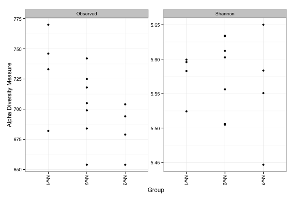
At this point we can compute the number of OTUs and the Shannon diversity index after the rarefaction:

> # rarefy without replacement
> ps.rarefied = rarefy_even_depth(ps, rngseed=1, sample.size=0.9*min(sample_sums(ps)), replace=F)
> # plot alpha diversity indexes
> plot_richness(ps.rarefied, x="Group", measures=c("Observed", "Chao1", "Shannon"))

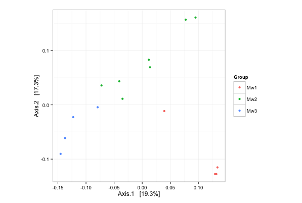
Finnaly, we can plot the PCoA on the unweighted UniFrac distance of samples:

> # PCoA plot on the unweighted UniFrac distance
> ordination = ordinate(ps.rarefied, method="PCoA", distance="unifrac", weighted=F)
> plot_ordination(ps.rarefied, ordination, color="Group") + theme(aspect.ratio=1)