An introduction to the downstream analysis with R and phyloseq¶

Note

This tutorial requires Paired-end sequencing - 97% OTU to be done.

Note

This tutorial requires R, phyloseq and ggplot2 (tested on R v3.4. and phyloseq v1.22.3) to be installed in your system.

We can import the micca processed data (the BIOM file, the phylogenetic tree and the representative sequences) into the R environment using the phyloseq library.

The import_biom() function allows to simultaneously import the BIOM file and an associated phylogenetic tree file and reference sequence file.

> library("phyloseq")
> library("ggplot2")
> setwd("denovo_greedy_otus") # set the working directory
> ps = import_biom("tables.biom", treefilename="tree_rooted.tree",
+ refseqfilename="otus.fasta")
> sample_data(ps)$Month <- as.numeric(sample_data(ps)$Month)
> ps
phyloseq-class experiment-level object
otu_table()   OTU Table:         [ 529 taxa and 34 samples ]
sample_data() Sample Data:       [ 34 samples by 4 sample variables ]
tax_table()   Taxonomy Table:    [ 529 taxa by 6 taxonomic ranks ]
phy_tree()    Phylogenetic Tree: [ 529 tips and 528 internal nodes ]
refseq()      DNAStringSet:      [ 529 reference sequences ]

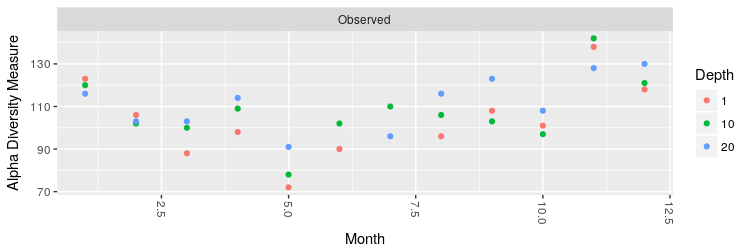
At this point, we can compute the number of OTUs as measure of alpha diversity after the rarefaction:

> # rarefy without replacement
> ps.rarefied = rarefy_even_depth(ps, rngseed=1, sample.size=0.9*min(sample_sums(ps)), replace=F)
> # plot the number of observed OTUs
> plot_richness(ps.rarefied, x="Month", color="Depth", measures=c("Observed"))

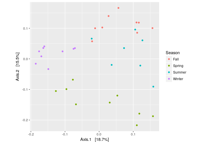
Finnaly, we can plot the PCoA using the unweighted UniFrac as distance:

> # PCoA plot using the unweighted UniFrac as distance
> ordination = ordinate(ps.rarefied, method="PCoA", distance="unifrac", weighted=F)
> plot_ordination(ps.rarefied, ordination, color="Season") + theme(aspect.ratio=1)