An introduction to the downstream analysis with R and phyloseq
Note
This tutorial requires Paired-end sequencing - 97% OTU to be done.
Note
This tutorial requires R, phyloseq ggplot2 and vegan (tested on R v3.4 and phyloseq v1.22.3) to be installed in your system.
Import data and preparation
We can import the micca processed data (the BIOM file, the phylogenetic tree and the representative sequences) into the R environment using the phyloseq library.
The import_biom() function allows to simultaneously import the BIOM
file and an associated phylogenetic tree file and reference sequence
file.
> library("phyloseq")
> library("ggplot2")
> library("vegan")
> setwd("denovo_greedy_otus") # set the working directory
> ps = import_biom("tables.biom", treefilename="tree_rooted.tree", refseqfilename="otus.fasta")
> sample_data(ps)$Month <- as.numeric(sample_data(ps)$Month)
> ps
phyloseq-class experiment-level object
otu_table()   OTU Table:         [ 529 taxa and 34 samples ]
sample_data() Sample Data:       [ 34 samples by 4 sample variables ]
tax_table()   Taxonomy Table:    [ 529 taxa by 6 taxonomic ranks ]
phy_tree()    Phylogenetic Tree: [ 529 tips and 528 internal nodes ]
refseq()      DNAStringSet:      [ 529 reference sequences ]
In this case, the phyloseq object includes the OTU table (which contains the OTU counts for each sample), the sample data matrix (containing the sample metadata), the taxonomy table (the predicted taxonomy for each OTU), the phylogenetic tree, and the OTU representative sequences.
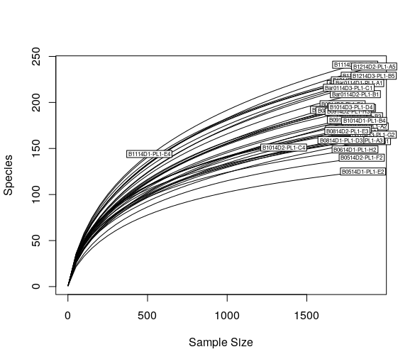
Now this point we can plot the rarefaction curves using vegan:
> rarecurve(t(otu_table(ps)), step=50, cex=0.5)
Now, we can rarefy in order to bring the samples to the same depth (in this case is the 90% of the abundance of the sample with less reads):
> # rarefy without replacement
> ps.rarefied = rarefy_even_depth(ps, rngseed=1, sample.size=0.9*min(sample_sums(ps)), replace=F)
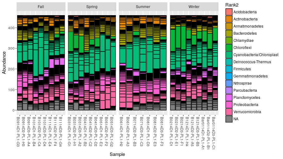
Plot abundances
Plot the abundances and color each OTU according its classified phylum (Rank2):
> plot_bar(ps.rarefied, fill="Rank2") + facet_wrap(~Season, scales = "free_x", nrow = 1)
Alternatively, we can merge the OTU at the phylum level and build a new phyloseq object:
> ps.phylum = tax_glom(ps.rarefied, taxrank = "Rank2", NArm = F)
> ps.phylum
phyloseq-class experiment-level object
otu_table()   OTU Table:         [ 35 taxa and 34 samples ]
sample_data() Sample Data:       [ 34 samples by 4 sample variables ]
tax_table()   Taxonomy Table:    [ 35 taxa by 6 taxonomic ranks ]
phy_tree()    Phylogenetic Tree: [ 35 tips and 34 internal nodes ]
refseq()      DNAStringSet:      [ 35 reference sequences ]
Now we can make the new bar plot at the class level:
> plot_bar(ps.phylum, fill="Rank2") + facet_wrap(~Season, scales = "free_x", nrow = 1)
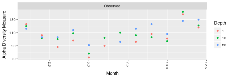
Alpha diversity
Now we can plot the number of observed OTUs in each month, coloring the values according to the sampling depth:
> plot_richness(ps.rarefied, x="Month", color="Depth", measures=c("Observed"))
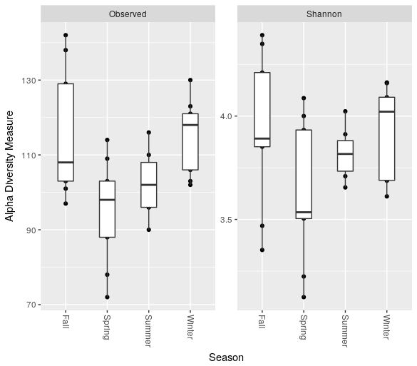
Moreover, we can make a boxplot of the number of OTUs and the Shannon entropy grouping the different months by season:
> plot_richness(ps.rarefied, x="Season", measures=c("Observed", "Shannon")) + geom_boxplot()
Beta diversity
Now, we can plot the PCoA using the unweighted UniFrac as distance:
> # PCoA plot using the unweighted UniFrac as distance
> wunifrac_dist = distance(ps.rarefied, method="unifrac", weighted=F)
> ordination = ordinate(ps.rarefied, method="PCoA", distance=wunifrac_dist)
> plot_ordination(ps.rarefied, ordination, color="Season") + theme(aspect.ratio=1)
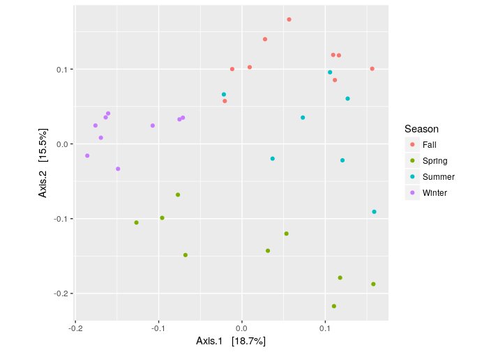
At this point, we test whether the seasons differ significantly from each other using the permutational ANOVA (PERMANOVA) analysis:
> adonis(wunifrac_dist~sample_data(ps.rarefied)$Season)

Call:
adonis(formula = wunifrac_dist ~ sample_data(ps.rarefied)$Season)

Permutation: free
Number of permutations: 999

Terms added sequentially (first to last)

                                Df SumsOfSqs  MeanSqs F.Model     R2 Pr(>F)
sample_data(ps.rarefied)$Season  3    0.6833 0.227765  4.3451 0.3029  0.001 ***
Residuals                       30    1.5726 0.052419         0.6971
Total                           33    2.2559                  1.0000
---
Signif. codes:  0 ‘***’ 0.001 ‘**’ 0.01 ‘*’ 0.05 ‘.’ 0.1 ‘ ’ 1