An introduction to the downstream analysis with R and phyloseq
In this tutorial we describe a R pipeline for the downstream analysis starting from the output of micca. In particular, we will discuss the following topics:
- rarefaction;
- taxonomy and relative abundances;
- alpha diversity and non-parametric tests;
- beta diversity and PERMANOVA;
- differential abundance testing with DESeq2.
You can download the script here.
Warning
- This tutorial requires Paired-end sequencing - 97% OTU to be done.
- The tutorial is tested on R 3.5.3, phyloseq 1.26.1, ggplot2 3.1.0, vegan 2.5-4 and DESeq2 1.22.2.
(Optional) Using the Dockerized RStudio environment
The tutorial can be run using a Docker image with
the required packages installed. Run the following command line mounting the
host working directory (i.e. the directory containing the micca output files, in
this case /Users/davide/micca) into the /home/rstudio/micca folder:
docker run --rm -d -p 8787:8787 -e DISABLE_AUTH=true --name rstudio-micca \
    -v /Users/davide/micca:/home/rstudio/micca \
    compmetagen/rstudio-micca
Open a browser and go to 127.0.0.1:8787.
Warning
Files stored outside the micca directory will be lost when you stop the
container.
You can stop (and destroy) the container using the following line:
docker stop rstudio-micca
Import data and preparation
Import the micca processed data (the BIOM file, the phylogenetic tree and the
representative sequences) into the R environment using the import_biom()
function available in phyloseq library.
> library("phyloseq")
> library("ggplot2")
> library("vegan")
> library("DESeq2")
> setwd("/home/rstudio/micca/garda/denovo_greedy_otus") # set the working directory
> ps = import_biom("tables.biom", treefilename="tree_rooted.tree", refseqfilename="otus.fasta")
> sample_data(ps)$Month <- as.numeric(sample_data(ps)$Month)
> ps
phyloseq-class experiment-level object
otu_table()   OTU Table:         [ 529 taxa and 34 samples ]
sample_data() Sample Data:       [ 34 samples by 4 sample variables ]
tax_table()   Taxonomy Table:    [ 529 taxa by 6 taxonomic ranks ]
phy_tree()    Phylogenetic Tree: [ 529 tips and 528 internal nodes ]
refseq()      DNAStringSet:      [ 529 reference sequences ]
The import_biom() function returns a phyloseq object which includes the OTU
table (which contains the OTU counts for each sample), the sample data matrix
(containing the metadata for each sample), the taxonomy table (the predicted
taxonomy for each OTU), the phylogenetic tree, and the OTU representative
sequences.
Print the metadata using the phyloseq function sample_data():
> sample_data(ps)
Sample Data:        [34 samples by 4 sample variables]:
                Season Depth Month Year
B0214D1-PL1-D1   Winter     1     2   14
B0214D2-PL1-E1   Winter    10     2   14
B0214D3-PL1-F1   Winter    20     2   14
B0314D1-PL1-G1   Spring     1     3   14
B0314D2-PL1-H1   Spring    10     3   14
B0314D3-PL1-A2   Spring    20     3   14
B0414D1-PL1-B2   Spring     1     4   14
B0414D2-PL1-C2   Spring    10     4   14
B0414D3-PL1-D2   Spring    20     4   14
B0514D1-PL1-E2   Spring     1     5   14
B0514D2-PL1-F2   Spring    10     5   14
B0514D3-PL1-G2   Spring    20     5   14
B0614D1-PL1-H2   Summer     1     6   14
B0614D2-PL1-A3   Summer    10     6   14
B0714D2-PL1-B3   Summer    10     7   14
B0714D3-PL1-C3   Summer    20     7   14
B0814D1-PL1-D3   Summer     1     8   14
B0814D2-PL1-E3   Summer    10     8   14
B0814D3-PL1-F3   Summer    20     8   14
B0914D1-PL1-G3     Fall     1     9   14
B0914D2-PL1-H3     Fall    10     9   14
B0914D3-PL1-A4     Fall    20     9   14
B1014D1-PL1-B4     Fall     1    10   14
B1014D2-PL1-C4     Fall    10    10   14
B1014D3-PL1-D4     Fall    20    10   14
B1114D1-PL1-E4     Fall     1    11   14
B1114D2-PL1-F4     Fall    10    11   14
B1114D3-PL1-G4     Fall    20    11   14
B1214D1-PL1-H4   Winter     1    12   14
B1214D2-PL1-A5   Winter    10    12   14
B1214D3-PL1-B5   Winter    20    12   14
Bar0114D1-PL1-A1 Winter     1     1   14
Bar0114D2-PL1-B1 Winter    10     1   14
Bar0114D3-PL1-C1 Winter    20     1   14
The sample data contains 4 features for each sample: the season of sampling, the sampling depth (in m), the month and the year of sampling .
Plot the rarefaction curves using vegan function rarecurve():
> rarecurve(t(otu_table(ps)), step=50, cex=0.5)
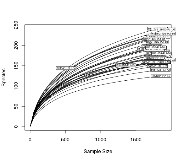
otu_table() is a phyloseq function which extract the OTU table from the
phyloseq object.
Rarefy the samples without replacement. Rarefaction is used to simulate even number of reads per sample. In this example, the rarefaction depth chosen is the 90% of the minimum sample depth in the dataset (in this case 459 reads per sample).
> # rarefy without replacement
> ps.rarefied = rarefy_even_depth(ps, rngseed=1, sample.size=0.9*min(sample_sums(ps)), replace=F)
Warning
- Rarefaction can waste a lot of data and would not be necessary. See https://doi.org/10.1371/journal.pcbi.1003531.
- Remember to set the random seed (
rngseed) for repeatable experiments.
Exercise
Plot the samples depths before and after the rarefaction using the
phyloseq function sample_sums().
Plot abundances
Using the rarefied dataset, make a stacked barplot of the abundances (read
counts) and color each OTU (i.e. each bar) according its classified phylum (in
this case Rank2):
> plot_bar(ps.rarefied, fill="Rank2")
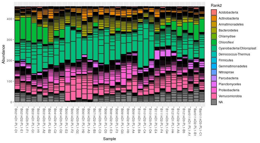
The plot_bar() function returns a ggplot2 object that can be customized
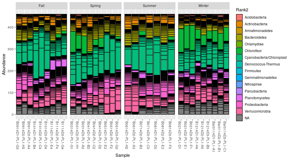
with additional options, in this case we separate the samples in 4 panels
according to the season:
> plot_bar(ps.rarefied, fill="Rank2") + facet_wrap(~Season, scales="free_x", nrow=1)
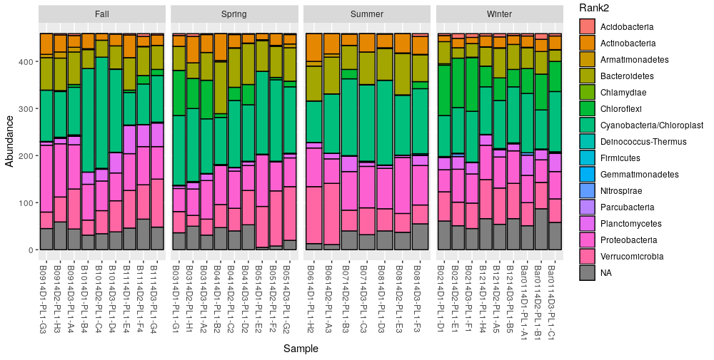
Alternatively, we can merge the OTUs at the phylum level and build a new phyloseq
object. Given a taxonomic rank (in this case the phylum), the phyloseq function
tax_glom merges the OTUs with the same taxonomy, summing the abundances:
> ps.phylum = tax_glom(ps.rarefied, taxrank="Rank2", NArm=FALSE)
> ps.phylum
phyloseq-class experiment-level object
otu_table()   OTU Table:         [ 35 taxa and 34 samples ]
sample_data() Sample Data:       [ 34 samples by 4 sample variables ]
tax_table()   Taxonomy Table:    [ 35 taxa by 6 taxonomic ranks ]
phy_tree()    Phylogenetic Tree: [ 35 tips and 34 internal nodes ]
refseq()      DNAStringSet:      [ 35 reference sequences ]
The option NArm set to FALSE forces the function to keep the
unclassified OTUs at the phylum level. Now we can make a cleaner bar plot:
> plot_bar(ps.phylum, fill="Rank2") + facet_wrap(~Season, scales= "free_x", nrow=1)
Exercise
Make a stacked barplot at class level (Rank3).
Alpha diversity
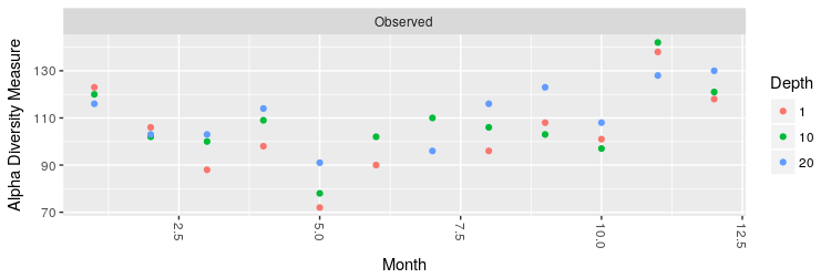
Plot the number of OTUs at each month coloring the points according to the sampling depth:
> plot_richness(ps.rarefied, x="Month", color="Depth", measures=c("Observed"))
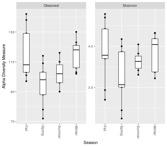
Make a boxplot of the number of OTUs and the Shannon entropy grouping the different months by season:
> plot_richness(ps.rarefied, x="Season", measures=c("Observed", "Shannon")) + geom_boxplot()
We can export a data.frame containig a number of standard alpha diversity
estimates using the phyloseq function estimate_richness()
> rich = estimate_richness(ps.rarefied)
> rich
                Observed    Chao1 se.chao1      ACE    se.ACE  Shannon   Simpson InvSimpson   Fisher
B0214D1.PL1.D1        106 197.8667 35.57985 188.3066  8.170040 3.687611 0.9299652   14.27862 43.21532
B0214D2.PL1.E1        102 143.1304 16.39579 161.0871  6.968287 3.689071 0.9314271   14.58303 40.65808
B0214D3.PL1.F1        103 184.0588 30.82336 190.4337  7.690088 3.611560 0.9227125   12.93871 41.28956
B0314D1.PL1.G1         88 137.4000 21.40127 142.2737  6.479689 3.534831 0.9325188   14.81895 32.34465
B0314D2.PL1.H1        100 222.7692 47.63464 203.5988  7.938369 3.504056 0.9304873   14.38587 39.41058
B0314D3.PL1.A2        103 178.2000 30.13564 160.8535  6.547177 3.787005 0.9486475   19.47324 41.28956
B0414D1.PL1.B2         98 143.0000 20.26436 136.2743  5.823351 4.086749 0.9750571   40.09153 38.18345
B0414D2.PL1.C2        109 224.9091 47.96245 172.8367  7.082246 4.000190 0.9664754   29.82883 45.18882
B0414D3.PL1.D2        114 186.5455 26.01395 211.5217  8.993286 3.932662 0.9602954   25.18601 48.58680
B0514D1.PL1.E2         72  99.1875 13.13050 109.1346  6.234068 3.124113 0.9126215   11.44446 23.97705
B0514D2.PL1.F2         78 109.1667 14.13628 122.0444  6.234465 3.223947 0.9125835   11.43949 26.97943
B0514D3.PL1.G2         91 128.0588 16.43157 126.6355  5.731954 3.524923 0.9258547   13.48704 34.04531
B0614D1.PL1.H2         90 123.0000 15.00832 128.4771  5.792422 3.816668 0.9577323   23.65873 33.47364
B0614D2.PL1.A3        102 151.2857 19.37303 167.6238  7.074761 3.757622 0.9423821   17.35571 40.65808
B0714D2.PL1.B3        110 172.6364 23.12117 187.8670  8.028159 3.709128 0.9258547   13.48704 45.85743
B0714D3.PL1.C3         96 141.5556 19.02400 151.4630  6.818280 3.850288 0.9634946   27.39319 36.97645
B0814D1.PL1.D3         96 178.5000 34.94025 155.8289  6.447118 3.654719 0.9326233   14.84192 36.97645
B0814D2.PL1.E3        106 155.5000 19.71247 162.2091  6.744816 4.022988 0.9689815   32.23887 43.21532
B0814D3.PL1.F3        116 216.6471 36.87625 215.7956  8.770340 3.911931 0.9456952   18.41456 49.98502
B0914D1.PL1.G3        108 168.2727 22.42221 201.5552  9.294336 3.891102 0.9617763   26.16180 44.52562
B0914D2.PL1.H3        103 162.3684 23.12990 180.7485  8.445071 3.886107 0.9643964   28.08706 41.28956
B0914D3.PL1.A4        123 178.0000 19.47167 199.4132  8.292517 4.090999 0.9670545   30.35312 55.06042
B1014D1.PL1.B4        101 173.5263 27.19010 193.4237  8.337151 3.469170 0.9060428   10.64314 40.03176
B1014D2.PL1.C4         97 251.0000 63.34083 207.5726  8.807031 3.352156 0.8968440    9.69406 37.57745
B1014D3.PL1.D4        108 180.0588 27.98694 171.2683  6.839082 3.851583 0.9479830   19.22447 44.52562
B1114D1.PL1.E4        138 244.6364 35.62005 235.2076  8.598060 4.349086 0.9764620   42.48457 66.94886
B1114D2.PL1.F4        142 217.6774 24.31684 250.3584  9.765194 4.391405 0.9794808   48.73491 70.36907
B1114D3.PL1.G4        129 206.5385 26.10650 225.4320  8.773816 4.210509 0.9742881   38.89256 59.64440
B1214D1.PL1.H4        118 240.0625 44.22653 241.1003  9.310808 4.091076 0.9714972   35.08426 51.40601
B1214D2.PL1.A5        121 185.5652 23.38079 199.4590  8.499590 4.159264 0.9720763   35.81183 53.58096
B1214D3.PL1.B5        130 256.1364 40.94272 298.4156 10.584524 4.162425 0.9733673   37.54785 60.43014
Bar0114D1.PL1.A1      123 190.7778 23.19105 215.1598  8.974270 4.021200 0.9614251   25.92359 55.06042
Bar0114D2.PL1.B1      120 216.3158 34.30966 222.7492  9.064837 4.028745 0.9586721   24.19674 52.85012
Bar0114D3.PL1.C1      116 187.8696 25.47702 221.1842  8.864324 3.932334 0.9560141   22.73454 49.98502
Test whether the observed number of OTUs differs significantly between seasons. We make a non-parametric test, the Wilcoxon rank-sum test (Mann-Whitney):
> pairwise.wilcox.test(rich$Observed, sample_data(ps.rarefied)$Season)

    Pairwise comparisons using Wilcoxon rank sum test

data:  rich$Observed and metasample_data(ps.rarefied)data$Season

       Fall  Spring Summer
Spring 0.112 -      -
Summer 0.270 0.681  -
Winter 1.000 0.025  0.112

P value adjustment method: holm
By default, the function pairwise.wilcox.test() reports the pairwise
adjusted (Holm) p-values.
Exercise
Repeat the test on the Shannon indexes.
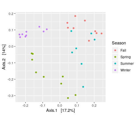
Beta diversity
Plot the PCoA using the unweighted UniFrac as distance:
> # PCoA plot using the unweighted UniFrac as distance
> wunifrac_dist = phyloseq::distance(ps.rarefied, method="unifrac", weighted=F)
> ordination = ordinate(ps.rarefied, method="PCoA", distance=wunifrac_dist)
> plot_ordination(ps.rarefied, ordination, color="Season") + theme(aspect.ratio=1)
Test whether the seasons differ significantly from each other using the permutational ANOVA (PERMANOVA) analysis:
> adonis(wunifrac_dist ~ sample_data(ps.rarefied)$Season)

Call:
adonis(formula = wunifrac_dist ~ sample_data(ps.rarefied)$Season)

Permutation: free
Number of permutations: 999

Terms added sequentially (first to last)

                                Df SumsOfSqs MeanSqs F.Model      R2 Pr(>F)
sample_data(ps.rarefied)$Season  3    1.3011 0.43372  4.1604 0.29381  0.001 ***
Residuals                       30    3.1274 0.10425         0.70619
Total                           33    4.4286                 1.00000
---
Signif. codes:  0 ‘***’ 0.001 ‘**’ 0.01 ‘*’ 0.05 ‘.’ 0.1 ‘ ’ 1
Exercise
Make the PCoA and the PERMANOVA using the Bray-Curtis dissimilarity instead.
OTU differential abundance testing with DESeq2
To test the differences at OTU level between seasons using DESeq2, we need to
convert the Season column into factor. Note that we use the data without
rarefaction (i.e. ps object):
> sample_data(ps)$Season <- as.factor(sample_data(ps)$Season)
Convert the phyloseq object to a DESeqDataSet and run DESeq2:
> ds = phyloseq_to_deseq2(ps, ~ Season)
> ds = DESeq(ds)
Extract the result table from the ds object usind the DESeq2 function
results and filter the OTUs using a False Discovery Rate (FDR) cutoff of
0.01. In this example we return the significantly differentially abundant OTU
between the seasons “Spring” and “Fall”:
> alpha = 0.01
> res = results(ds, contrast=c("Season", "Spring", "Fall"), alpha=alpha)
> res = res[order(res$padj, na.last=NA), ]
> res_sig = res[(res$padj < alpha), ]
> res_sig
log2 fold change (MLE): Season Spring vs Fall
Wald test p-value: Season Spring vs Fall
DataFrame with 62 rows and 6 columns
                baseMean    log2FoldChange             lfcSE              stat               pvalue                 padj
                <numeric>         <numeric>         <numeric>         <numeric>            <numeric>            <numeric>
DENOVO17 22.7436598625802  -4.1529844728879 0.552035702386233 -7.52303601911288 5.35186717121325e-14 1.24163318372147e-11
DENOVO35 10.6015033917283 -7.36751901929925  1.01933372324247 -7.22777913779147 4.90956301343594e-13  5.6950930955857e-11
DENOVO91 5.31287448011852 -6.51255526618412 0.947998700432628 -6.86979345352695 6.42949270405053e-12 4.97214102446574e-10
DENOVO2  82.4704545010533 -4.14259840011034 0.673404296938788 -6.15172552201119 7.66444402875036e-10 4.44537753667521e-08
DENOVO7  15.6311735008548  5.91263059667889 0.979789881740526   6.0345903819455 1.59366414316775e-09 7.39460162429838e-08
...                   ...               ...               ...               ...                  ...                  ...
DENOVO83 3.63662006180492  1.92505847356698 0.617438877584007  3.11781221341228  0.00182198852945677  0.00728795411782707
DENOVO89 2.68296393708501  2.84137889985046 0.912892035548744  3.11250267195342  0.00185508334637251  0.00729456502302411
DENOVO72 4.86241695816352  2.71763740147229 0.895564240058129  3.03455327927775  0.00240892202480818  0.00931449849592497
DENOVO21  17.208142677795  -1.1266184329166 0.373108760004578 -3.01954430901804    0.002531552600065  0.00962820005270621
DENOVO55 6.24723247307275  2.09415598552554 0.695335908667259  3.01171845063975  0.00259773414843998  0.00972055358771089
The result table reports base means across samples, log2 fold changes, standard errors, test statistics, p-values and adjusted p-values.
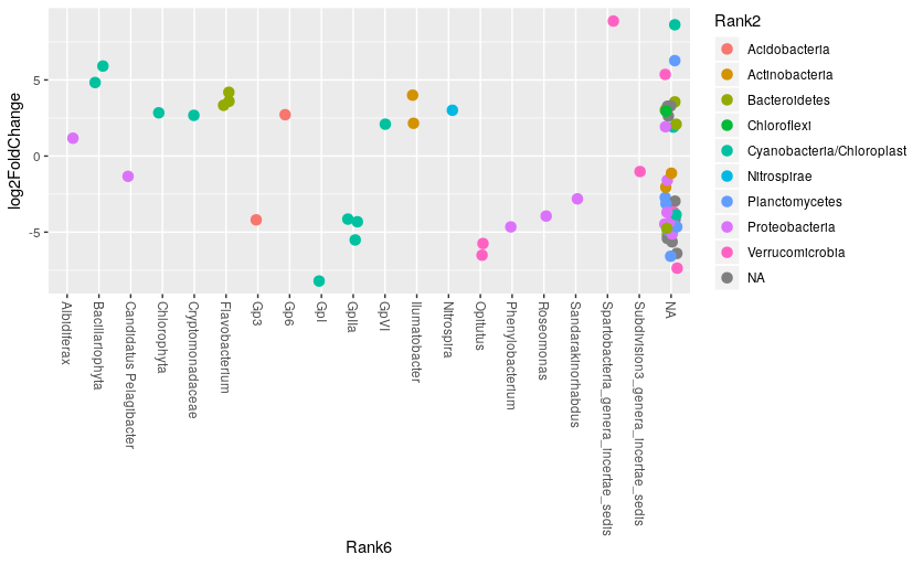
Make a genus vs log2FC plot of the significant OTUs:
> res_sig = cbind(as(res_sig, "data.frame"), as(tax_table(ps)[rownames(res_sig), ], "matrix"))
> ggplot(res_sig, aes(x=Rank6, y=log2FoldChange, color=Rank2)) +
    geom_jitter(size=3, width = 0.2) +
    theme(axis.text.x = element_text(angle = -90, hjust = 0, vjust=0.5))
Exercise
Test the differences between summer and fall and compare the results with those above.